Accuracy and performance

This page measures how accurate tensorderiv’s operators are on scattered points, how noise and the number of neighbours affect them, and how fast stencils and operators are computed. Every figure is computed when the page is built, against the tensorderiv in the repository.

All accuracy tests use the same smooth field on random points in the unit square, and measure the median error over the points at least 0.1 from the boundary, since stencils at the boundary are one-sided (the user guide shows that effect separately):

import time                                            # for timing
import numpy as np                                     # arrays
import matplotlib.pyplot as plt                        # plotting
import tensorderiv as td                               # the package

def field(points):
    # A smooth 2D test field, sin(3x)·exp(y) + cos(2y), with its exact gradient and Laplacian
    x, y = points.T                                    # the coordinate columns
    f = np.sin(3 * x) * np.exp(y) + np.cos(2 * y)
    grad = np.column_stack([3 * np.cos(3 * x) * np.exp(y),
                            np.sin(3 * x) * np.exp(y) - 2 * np.sin(2 * y)])
    lap = -8 * np.sin(3 * x) * np.exp(y) - 4 * np.cos(2 * y)
    return f, grad, lap

def interior(points, margin=0.1):
    # The points at least `margin` away from the boundary of the unit square
    return np.all((points > margin) & (points < 1 - margin), axis=1)

Convergence

Figure 1 shows the errors as the number of points grows. Each fourfold increase halves the spacing between points in 2D, so first-order methods halve their error and second-order methods quarter it. Both orders converge as designed, for the gradient and the Laplacian alike.

For comparison, the figure includes NumPy’s np.gradient with the same number of points arranged on a regular grid, where it uses second-order central differences. tensorderiv’s second-order gradient on scattered points converges at the same rate, with an error only about 2.5 times larger: scattered points cost little accuracy.

rng = np.random.default_rng(0)                         # reproducible random points
sizes = [1_000, 4_000, 16_000, 64_000]                 # numbers of points; each step halves the spacing
errors = {}                                            # median interior errors, one list per method
for n in sizes:
    points = rng.random((n, 2))                        # scattered points in the unit square
    f, grad, lap = field(points)
    inner = interior(points)
    for order in (1, 2):
        stencils = td.StencilSet(points, order=order)
        grad_error = np.linalg.norm(td.gradient(stencils, f) - grad, axis=1)  # error per point
        lap_error = np.abs(td.laplacian(stencils, f) - lap)
        errors.setdefault(("gradient", order), []).append(np.median(grad_error[inner]))
        errors.setdefault(("Laplacian", order), []).append(np.median(lap_error[inner]))
    # the same number of points on a regular grid, differentiated by np.gradient
    m = int(round(np.sqrt(n)))                         # grid points per axis
    axis = np.linspace(0.0, 1.0, m)
    gx, gy = np.meshgrid(axis, axis, indexing="ij")    # the grid's coordinates
    grid_points = np.column_stack([gx.ravel(), gy.ravel()])
    gf, ggrad, _ = field(grid_points)
    dfx, dfy = np.gradient(gf.reshape(m, m), axis, axis)  # second-order central differences
    grid_error = np.linalg.norm(np.column_stack([dfx.ravel(), dfy.ravel()]) - ggrad, axis=1)
    errors.setdefault(("gradient", "grid"), []).append(np.median(grid_error[interior(grid_points)]))

fig, axes = plt.subplots(1, 2, figsize=(10, 4), sharey=True)  # gradient left, Laplacian right
n = np.array(sizes, dtype=float)
for ax, quantity in zip(axes, ["gradient", "Laplacian"]):
    ax.loglog(n, errors[(quantity, 1)], "o-", color="tab:orange", label="order 1")
    ax.loglog(n, errors[(quantity, 2)], "o-", color="tab:blue", label="order 2")
    if quantity == "gradient":
        ax.loglog(n, errors[(quantity, "grid")], "s--", color="tab:green", label="np.gradient on a grid")
    ax.loglog(n, errors[(quantity, 1)][0] * (n / n[0]) ** -0.5, color="grey", lw=0.8)  # first order
    ax.loglog(n, errors[(quantity, 2)][0] * (n / n[0]) ** -1.0, color="grey", lw=0.8)  # second order
    ax.set_title(quantity)
    ax.set_xlabel("number of points")
axes[0].set_ylabel("median interior error")
axes[0].legend()
fig.tight_layout()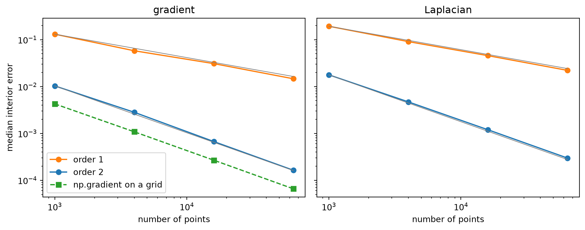

Figure 1: Median interior error against the number of points, for first- and second-order stencils on random points, and for np.gradient on a regular grid with the same number of points. The grey lines show first-order (N^(-1/2)) and second-order (N^(-1)) convergence.

Noise

Like every derivative estimate, the operators amplify noise in the field values. The weights grow as 1/h^2 with the stencil radius h, so noise of size \sigma in the values becomes an error of roughly \sigma/h in the gradient. Figure 2 adds Gaussian noise to the field on 40000 points. For second order, the method’s own error dominates up to a noise level of about 10^{-5}, and the noise above it; first order, whose own error is larger, tolerates noise up to about 10^{-4}. At every noise level, second order is never worse than first order, because its larger stencils average over more neighbours.

Two practical consequences follow. Finer point clouds amplify noise more, since h is smaller. And noisy data are best smoothed before differentiating, if precise derivatives are needed.

rng = np.random.default_rng(1)                         # reproducible points and noise
points = rng.random((40_000, 2))                       # 40000 scattered points
f, grad, _ = field(points)
inner = interior(points)
noise_levels = np.array([1e-6, 1e-5, 1e-4, 1e-3, 1e-2])  # standard deviations of the noise
noise = rng.standard_normal(len(points))               # one noise sample, scaled to each level

fig, ax = plt.subplots(figsize=(6, 4))                 # one panel
for order, colour in [(1, "tab:orange"), (2, "tab:blue")]:
    stencils = td.StencilSet(points, order=order)
    error = [np.median(np.linalg.norm(td.gradient(stencils, f + s * noise) - grad, axis=1)[inner])
             for s in noise_levels]                    # error at each noise level
    ax.loglog(noise_levels, error, "o-", color=colour, label=f"order {order}")
ax.loglog(noise_levels, 80 * noise_levels, color="grey", lw=0.8)  # proportional to the noise
ax.set_xlabel("noise standard deviation")
ax.set_ylabel("median interior gradient error")
ax.legend()
fig.tight_layout()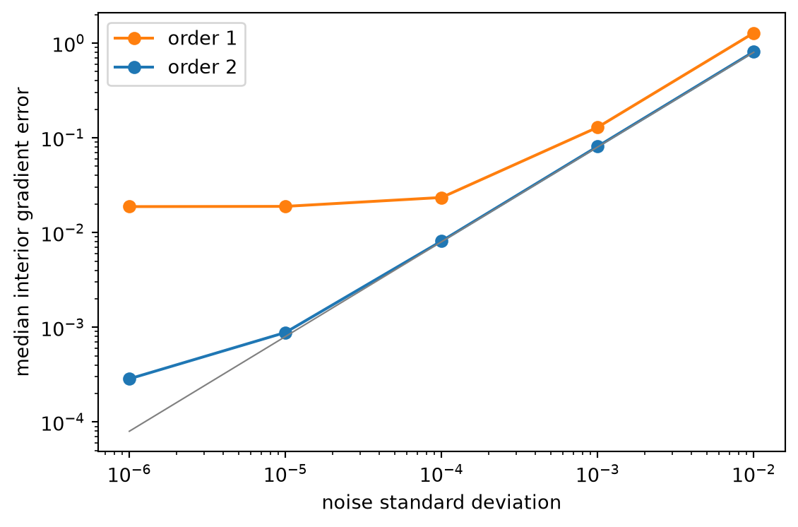

Figure 2: Median interior gradient error against the standard deviation of noise added to the field values, on 40000 random points. The grey line is proportional to the noise.

Number of neighbours

The default number of neighbours is twice the minimum for the order and dimension. Figure 3 shows why. At the minimum itself, the stencils are ill-conditioned, and the worst errors are large. Beyond it, the two orders behave differently. First order keeps improving with more neighbours, because its error comes from the third moment of the stencil, which averages out as stencils grow more symmetric. Second order has cancelled that moment already, so a larger stencil radius only adds error; its typical error is lowest somewhat below the default, but the worst errors are smallest near the default.

factors = [1.2, 1.5, 2.0, 2.5, 3.0, 4.0, 5.0]          # numbers of neighbours, as multiples of the minimum

fig, ax = plt.subplots(figsize=(6, 4))                 # one panel
for order, colour in [(1, "tab:orange"), (2, "tab:blue")]:
    k_min = td.minimum_neighbours(2, order)            # the minimum for this order in 2D
    ks = [int(round(factor * k_min)) for factor in factors]
    median, worst = [], []
    for k in ks:
        stencils = td.StencilSet(points, order=order, k=k)
        error = np.linalg.norm(td.gradient(stencils, f) - grad, axis=1)  # error per point
        median.append(np.median(error[inner]))         # typical interior error
        worst.append(np.percentile(error, 99.9))       # the worst 0.1 %, boundary included
    multiples = np.array(ks) / k_min
    ax.semilogy(multiples, median, "o-", color=colour, label=f"order {order}: median")
    ax.semilogy(multiples, worst, "o--", color=colour, label=f"order {order}: worst 0.1 %")
ax.axvline(2.0, color="grey", lw=0.8)                  # the default
ax.set_xlabel("neighbours, as a multiple of the minimum")
ax.set_ylabel("gradient error")
ax.legend()
fig.tight_layout()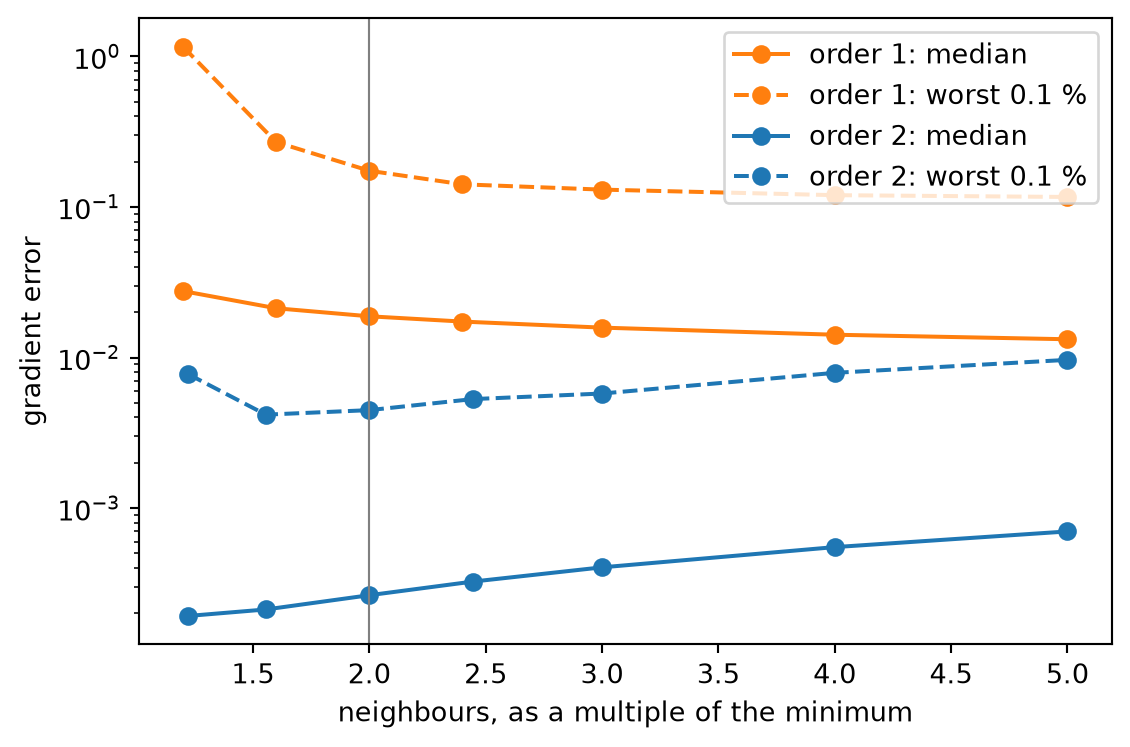

Figure 3: Gradient error against the number of neighbours, as a multiple of the minimum, on 40000 random points: the median over interior points (solid) and the worst 0.1 % over all points (dashed).

Speed

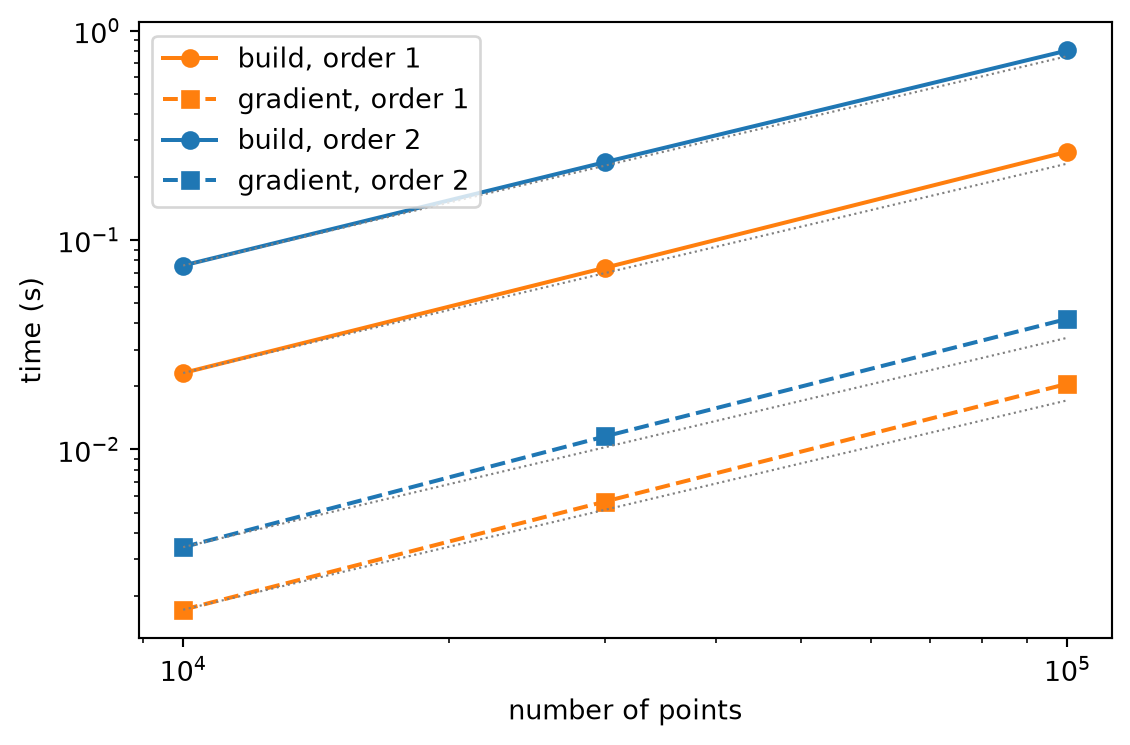
Figure 4 shows how long building the stencils and computing a gradient take, for point clouds in 3D. Both grow linearly with the number of points. The build includes SciPy’s neighbour search and all the weights; it is the expensive step, and is done once per point cloud. The operators then cost far less, so one StencilSet can serve any number of fields.

The times are measured on the machine that built this page, at build time, using all its cores. On a 20-core desktop CPU, building second-order stencils for 100000 points in 3D takes about 0.13 seconds, and the gradient of a vector field on them about 7 milliseconds.

def best_time(function, repeats=3):
    # the fastest of a few runs, which filters out one-off delays
    times = []
    for _ in range(repeats):
        start = time.perf_counter()
        function()
        times.append(time.perf_counter() - start)
    return min(times)

rng = np.random.default_rng(2)                         # reproducible random points
sizes = [10_000, 30_000, 100_000]                      # numbers of points
td.StencilSet(rng.random((1_000, 3)))                  # warm up once, so start-up costs are excluded
timings = {}
for n in sizes:
    points = rng.random((n, 3))                        # scattered points in the unit cube
    vector = np.column_stack([np.sin(points[:, 0]), points[:, 1] ** 2, points[:, 2]])  # a vector field
    for order in (1, 2):
        timings.setdefault(("build", order), []).append(
            best_time(lambda: td.StencilSet(points, order=order)))
        stencils = td.StencilSet(points, order=order)
        timings.setdefault(("gradient", order), []).append(
            best_time(lambda: td.gradient(stencils, vector)))

fig, ax = plt.subplots(figsize=(6, 4))                 # one panel
n = np.array(sizes, dtype=float)
for (step, order), times in timings.items():
    colour = "tab:orange" if order == 1 else "tab:blue"
    style = "o-" if step == "build" else "s--"
    ax.loglog(n, times, style, color=colour, label=f"{step}, order {order}")
    ax.loglog(n, times[0] * n / n[0], ":", color="grey", lw=0.8)  # proportional to the number of points
ax.set_xlabel("number of points")
ax.set_ylabel("time (s)")
ax.legend()
fig.tight_layout()

Figure 4: Time to build the stencils and to compute the gradient of a vector field, against the number of points in 3D, on the machine that built this page. The dotted lines are proportional to the number of points.