import numpy as np                                     # arrays
import tensorderiv as td                               # the package

np.set_printoptions(suppress=True)                     # print small numbers without exponents
rng = np.random.default_rng(1)                         # reproducible random numbers
points = rng.random((5_000, 3))                        # 5000 scattered points in the unit cube, one row per point
x, y, z = points.T # the coordinate columnsUser guide
This guide covers everything tensorderiv offers: building stencils, the fields the operators accept, evaluating at selected points, chaining derivatives, threading, and the method’s limitations. The examples below run in order and share their variables, starting from a cloud of random points:
Building stencils
A StencilSet finds each point’s nearest neighbours and computes their weights, once. Every operator then reuses it, for any number of fields sampled at the same points:
stencils = td.StencilSet(points)                       # second order, twice the minimum number of neighbours
print(stencils)                                        # a short summary
print(stencils.neighbours.shape, stencils.weights.shape)  # one row of neighbours and weights per point
StencilSet(5000 points in 3D, order=2, k=38)
(5000, 38) (5000, 38)StencilSet takes three optional arguments:
order:2by default, which makes every operator second-order accurate.1gives first-order operators from smaller stencils, which suits small point clouds or cheaper builds.k: the number of neighbours per point. The default is twice the minimum for the order and dimension, whichminimum_neighboursreports.threaded:Trueby default; see Threading.
first_order = td.StencilSet(points, order=1)           # first order: smaller stencils, cheaper to build
wider = td.StencilSet(points, k=60)                    # second order with 60 neighbours per point
print(first_order, wider, sep="\n")
print("minimum neighbours in 3D:", td.minimum_neighbours(3, 1), "(order 1),",
      td.minimum_neighbours(3, 2), "(order 2)")
StencilSet(5000 points in 3D, order=1, k=18)
StencilSet(5000 points in 3D, order=2, k=60)
minimum neighbours in 3D: 9 (order 1), 19 (order 2)The attributes points, neighbours and weights are plain NumPy arrays with one row per point. The neighbours of each point are sorted nearest first and never include the point itself.
Fields and their shapes
A field holds one value per point along its first axis: a number for a scalar field, a vector for a vector field, a matrix for a matrix field, and so on. The operators keep that point axis first:
| Field | values |
gradient |
divergence |
curl (3D) |
laplacian |
|---|---|---|---|---|---|
| Scalar | (P,) |
(P, N) |
– | – | (P,) |
| Vector | (P, N) |
(P, N, N) |
(P,) |
(P, N) |
(P, N) |
| Matrix | (P, N, m) |
(P, N, N, m) |
(P, m) |
(P, N, m) |
(P, N, m) |
Here P is the number of points and N the spatial dimension. Fields of higher rank follow the same pattern.
f = np.sin(x) * np.exp(y)                              # scalar field: one value per point
v = np.column_stack([x * y, np.sin(z), x**2 * z])      # vector field: one row of three per point
M = np.stack([v, 2 * v], axis=2)                       # matrix field: a 3 × 2 matrix per point

print("gradient of f:  ", td.gradient(stencils, f).shape)    # (points, 3)
print("gradient of v:  ", td.gradient(stencils, v).shape)    # (points, 3, 3)
print("gradient of M:  ", td.gradient(stencils, M).shape)    # (points, 3, 3, 2)
print("divergence of v:", td.divergence(stencils, v).shape)  # (points,)
print("divergence of M:", td.divergence(stencils, M).shape)  # (points, 2)
print("curl of v:      ", td.curl(stencils, v).shape)        # (points, 3)
print("laplacian of M: ", td.laplacian(stencils, M).shape)   # (points, 3, 2)
gradient of f: (5000, 3)
gradient of v: (5000, 3, 3)
gradient of M: (5000, 3, 3, 2)
divergence of v: (5000,)
divergence of M: (5000, 2)
curl of v: (5000, 3)
laplacian of M: (5000, 3, 2)Three conventions follow from the layout:
- The gradient puts the derivative direction right after the point index:
gradient(stencils, v)[p, a, j]is \partial v_j / \partial x_a at pointp. For a vector field, this is the transpose of the usual Jacobian. - The divergence contracts the derivative direction with the field’s first axis after the points, which must therefore have length
N. For a matrix field, it gives \sum_a \partial M_{aj} / \partial x_a for each columnj. - The curl takes the cross product with the field’s first axis after the points, which must have length 3, and only exists in three dimensions.
Evaluating at selected points
Every operator takes an optional at argument, which selects points exactly as NumPy indexing does. A single index leaves out the point axis, so a scalar result is a plain number. Only the selected points are computed:
print(td.gradient(stencils, f, at=0))                  # one point: no point axis, shape (3,)
print(td.gradient(stencils, f, at=[0, 1, 2]).shape)    # a list of points: shape (3, 3)
print(td.divergence(stencils, v, at=-1))               # negative indices count from the end
print(td.laplacian(stencils, f, at=slice(0, 1000)).shape)  # a slice: the first 1000 points
near_origin = np.linalg.norm(points, axis=1) < 0.3    # a boolean mask: points near the origin
print(td.gradient(stencils, f, at=near_origin).shape)  # only those points
[2.26030302 1.26137295 0.00087607]
(3, 3)
1.1256603632484903
(1000,)
(92, 3)Chaining derivatives
The gradient of any field is itself a field, so derivatives can be chained. The Hessian of a scalar field, for example, is the gradient of its gradient:
H = td.gradient(stencils, td.gradient(stencils, f))   # the Hessian: H[p, a, b] = ∂²f/∂x_a∂x_b
p = 2_000                                              # look at one interior point
exact = np.exp(y[p]) * np.array([[-np.sin(x[p]), np.cos(x[p]), 0],
                                 [np.cos(x[p]), np.sin(x[p]), 0],
                                 [0, 0, 0]])           # the exact Hessian of sin(x)·exp(y)
print("point:", points[p].round(3))
print("estimated:\n", H[p].round(3))
print("exact:\n", exact.round(3))
point: [0.387 0.452 0.81 ]
estimated:
[[-0.594 1.46 0.003]
[ 1.457 0.592 -0.001]
[-0.001 0.004 0.003]]
exact:
[[-0.593 1.456 0. ]
[ 1.456 0.593 0. ]
[ 0. 0. 0. ]]Each chained operator adds its own error, so a direct operator is preferable where one exists. The Laplacian is the main example: laplacian is markedly more accurate than the divergence of the gradient, because it uses the stencil once instead of twice. The exact Laplacian of \sin(x)\,e^y is zero:
lap = td.laplacian(stencils, f)                        # the Laplacian directly
div_grad = td.divergence(stencils, td.gradient(stencils, f))  # the divergence of the gradient
inner = np.all((points > 0.2) & (points < 0.8), axis=1)  # points away from the boundary
print("median error of laplacian:         ", np.median(np.abs(lap[inner])).round(5))
print("median error of divergence(grad):  ", np.median(np.abs(div_grad[inner])).round(5))
median error of laplacian: 0.00054
median error of divergence(grad): 0.00527Choosing the order and the number of neighbours
The default, second order with twice the minimum number of neighbours, is the right choice for almost all uses. It is roughly ten times more accurate than first order at the same resolution, and it stays ahead even when the field values carry noise. The accuracy page shows both in detail.
First order is worth considering when the point cloud is small, since second order needs at least 19 neighbours per point in 3D, or when building the stencils must be as cheap as possible. First order also benefits from more neighbours than the default, at proportional cost, whereas second order is most accurate near its default.
Threading
StencilSet and all four operators use every core by default. thread_count reports how many threads the Rust core uses. Pass threaded=False when calling tensorderiv from code that is already parallel, to avoid running more threads than there are cores. Threading never changes the results:
print("threads:", td.thread_count())                   # how many threads the Rust core uses
serial = td.StencilSet(points, threaded=False)         # build on one thread, e.g. inside your own parallel code
print(np.array_equal(serial.weights, stencils.weights))  # threading never changes the results
threads: 4
TrueLimitations
Accuracy drops near the boundary. Points near the edge of the cloud have all their neighbours on one side, so their stencils are one-sided. Within about one stencil radius of the boundary, the errors grow several-fold, as Figure 1 shows for a field in the unit square. Second order is still far more accurate there than first order is anywhere.
Code
import matplotlib.pyplot as plt                        # plotting

rng = np.random.default_rng(2)                         # reproducible random numbers
flat = rng.random((40_000, 2))                         # 40000 scattered points in the unit square
g = np.sin(3 * flat[:, 0]) * np.exp(flat[:, 1])        # a smooth field
exact_grad = np.column_stack([3 * np.cos(3 * flat[:, 0]) * np.exp(flat[:, 1]),
                              np.sin(3 * flat[:, 0]) * np.exp(flat[:, 1])])  # its exact gradient
distance = np.min(np.minimum(flat, 1 - flat), axis=1)  # distance from each point to the boundary
bins = np.geomspace(1e-4, 0.5, 25)                     # distance bins, finer near the boundary
centres = np.sqrt(bins[:-1] * bins[1:])                # the middle of each bin, on a log scale
which = np.digitize(distance, bins) - 1                # the bin of every point

fig, ax = plt.subplots(figsize=(8, 4))                 # one panel
for order, colour in [(1, "tab:orange"), (2, "tab:blue")]:
    stencils_2d = td.StencilSet(flat, order=order)     # stencils of this order
    error = np.linalg.norm(td.gradient(stencils_2d, g) - exact_grad, axis=1)  # gradient error per point
    median = [np.median(error[which == b]) for b in range(len(centres))]      # typical error per bin
    worst = [np.percentile(error[which == b], 99) for b in range(len(centres))]  # worst 1 % per bin
    ax.plot(centres, median, color=colour, label=f"order {order}: median")
    ax.plot(centres, worst, color=colour, ls="--", label=f"order {order}: 99th percentile")
ax.set_xscale("log"); ax.set_yscale("log")             # both axes logarithmic
ax.set_xlabel("distance to the boundary")              # axis labels
ax.set_ylabel("gradient error")
ax.legend(loc="center left", bbox_to_anchor=(1.02, 0.5))  # the legend beside the plot
fig.tight_layout()                                     # make room for it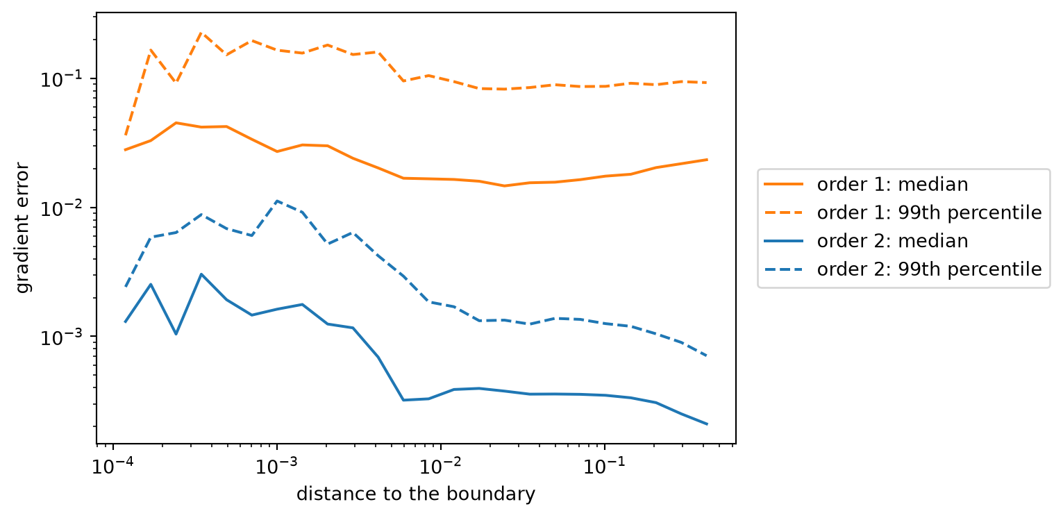
The points must fill their space. The weights need neighbours spread in every direction. Points on a curve or surface, such as a laser scan of an object, points on a sphere, or a plane embedded in 3D, cannot satisfy the moment conditions, and their derivatives would be meaningless. StencilSet checks every stencil and raises an error naming the first point that fails. For points on a plane, give their coordinates within the plane instead:
theta = rng.random(3_000) * 2 * np.pi                  # random longitudes
phi = np.arccos(rng.uniform(-1, 1, 3_000))             # random latitudes, evenly spread over the sphere
sphere = np.column_stack([np.sin(phi) * np.cos(theta),  # 3000 points on the unit sphere's surface
                          np.sin(phi) * np.sin(theta),
                          np.cos(phi)])
try:
    td.StencilSet(sphere)                              # stencils on a curved surface...
except ValueError as error:
    print(error)                                       # ...are refused, with the reason
point 0: the neighbours cannot satisfy the moment conditions (residual 3.0e0); they may lie on a curve or surface, or too few of them span every direction: try a larger k, or give the points in coordinates of their own dimensionRegular grids need enough neighbours at order 1. On a regular grid, the stencils at the faces see only a few layers of points. With the default order 2 this is no problem: the stencils there lose their second-order accuracy, as at any boundary, but stay correct. At order 1 in 3D, the default 18 neighbours are too few, and StencilSet raises the same error; 24 neighbours suffice.
Noise is amplified. Like every derivative estimate, the operators amplify noise in the field values: the weights grow as 1/h^2 with the stencil radius h, so a finer point cloud amplifies noise more. Smooth noisy data first if precise derivatives are needed.
Memory. A StencilSet stores k neighbour indices and k weights per point: about 600 MB for a million points in 3D at second order. The operators need little memory beyond their results.